5  Biochemical kinetics

Biochemical kinetics concern the concentration of chemical substances in biological systems. In this section we neglect spatial variation in concentrations, effectively assuming chemical reactions occur in environments that are “well-mixed”.

5.1 The law of mass action

We denote the \(i^{th}\) chemical species using the notation \(C_i\). The concentration of molecule type \(C_i\) is denoted \([C_i]\) and represents the number of molecules of \(C_i\) per unit volume.

Suppose \(C_1,..C_M\) undergo the reaction

\[ \lambda_1C_1+\lambda_2 C_2+...+\lambda_m C_M \xrightleftharpoons[k_{b}]{k_{f}} \gamma_1 C_1+\gamma_2 C_2 + ... \gamma_M C_M. \]

the law of mass action states that the forward reaction proceeds at rate

\[ k_f[C_1]^\lambda_1 [C_2]^\lambda_2 ..[C_M]^\lambda_M \]

whilst the backward reaction proceeds at rate

\[ k_b[C_1]^\gamma_1[C_2]^\gamma_2 ..[C_M]^\gamma_M \]

where \(k_f\) and \(k_b\) are dimensional rate constants.

Example

Suppose A and B react to produce C. Hence \[ A+B\xrightarrow{k} C. \]

The law of mass action states that the rate of the reaction is

\[ k[A][B]. \]

Using the reaction rates, we write down ordinary differential equations that describe how concentrations of a given molecule will change in time. Hence

\[ \frac{d[C]}{dt}=k[A][B]. \]

Example

Consider the reversible reaction \[ A+B \xrightleftharpoons[k_{-}]{k_{+}} C. \] Define dependent variables, identify reaction rates and derive ordinary differential equations that describe how concentrations evolved in time.

The dependent variables are: \[ [A](t), \ \ [B](t), \ \ [C](t) \].

Applying the law of mass action yields the reaction rates:

\[ k_+[A][B] \ \ \textrm{and} \ \ k_-[C]\].

The ODEs are

\[ \begin{aligned} \frac{d[A]}{dt}&=-k_+[A][B]+k_-[C], \nonumber\\ \frac{d[B]}{dt}&=-k_+[A][B]+k_-[C], \nonumber\\ \frac{d[C]}{dt}&=k_+[A][B]-k_-[C]. \nonumber \end{aligned} \]

For a given set of initial conditions, \[ [A](t=0)=[A]_0, \ \ \ [B](t=0)=[B]_0, \ \ \ [C](t=0)=[C]_0, \] the ODEs can be solved and hence the concentrations of the different molecules described as time evolves.

5.1.1 Example

The previous example have had stochiometric constants all set to unity (i.e. all reactions involved a molecules of one species interaction with one from another). Consider the reaction in which one molecule of species A with \(m\) of species B giving rise to \(n\) molecules of species B and \(p\) molecules of species C, i.e. \[ A+mB \xrightarrow{k_1} nB + pC. %X \underset{k_2}{\stackrel{k_1}{\rightleftharpoons}} Y \]

The law of mass action says that the rate of the forward reaction is \[ k_1[A][B]^m. \]

The governing ODEs are \[ \begin{aligned} \frac{d[A]}{dt}&=-k_1[A][B]^m, \nonumber\\ \frac{d[B]}{dt}&=(n-m)k_1[A][B]^m, \nonumber\\ \frac{d[C]}{dt}&=pk_1[A][B]^m. \nonumber \end{aligned} \]

Example

Consider the reversible reaction \[ A+A \xrightleftharpoons[k_{-}]{k_{+}} B. \] Define dependent variables, identify reaction rates and derive ordinary differential equations that describe how concentrations evolved in time.

The reaction rates are \[ k_+[A]^2 \] and \[ k_- [B]. \] The ODEs are \[ \begin{aligned} \frac{d[A]}{dt}&=-2k_+[A]^2+2k_- [B] , \nonumber\\ \frac{d[B]}{dt}&=k_+[A]^2-k_- [B], \end{aligned} \]

5.2 Enzyme kinetics

Biochemical reactions are often regulated by enzymes (substances that convert a substrate into another substrate). Consider a chemical reaction in which substrate, \(S\), reacts with an enzyme, \(E\), to form a complex, \(C\). Suppose the complex can either undergo the reverse reaction or go on to form a product, \(P\), with the release of the enzyme, i.e. \[ S+E \xrightleftharpoons[k_{-1}]{k_{1}} C \xrightarrow{k_2} P+E . \]

5.2.1 Deriving the model equations

For notational convenience we let lower case letter denote concentrations, i.e. 

\[ s(t)=[S](t), \ \ c(t)=[C](t) , \\ e(t)=[E](t), \\ p(t)=[P](t). \]

Applying the law of mass action the above enzyme kinetic scheme can be described by the system of ODES

\[ \begin{aligned} \frac{d s}{dt} &= -k_1 se + k_{-1}c, \nonumber \\ \frac{d e}{dt} &= -k_1 se + k_{-1}c +k_2 c, \nonumber\\ \frac{d c}{dt} &= k_1 se - k_{-1}c-k_2c, \nonumber \\ \frac{d p}{dt} &= k_2 c. \end{aligned} \tag{5.1}\]

We consider initial conditions such that at \(t=0\) the reaction has not yet started, i.e. there is no product or complex formed \[ s(0)=s_0, \ \ e(0)=e_0, \ \ c(0)=0, \ \ p(0)=0, \] where \(s_0\) and \(e_0\) represent the initial concentrations of substrate and enzyme, respectively.

5.2.2 Numerical solutions

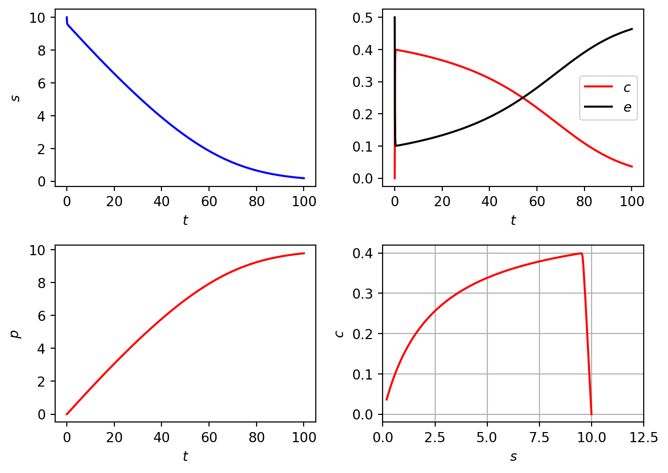
In Figure 5.1 we plot numerical solutions of Equation 5.1. For this solution we have chosen initial conditions such that \[ \frac{e_0}{s_0}\ll 1. \] Note that \(c\) and \(e\) evolve rapidly in time close to the initial data whilst those of \(s\) and \(p\) do not.

import numpy as np
import matplotlib.pyplot as plt
import scipy
from scipy.integrate import odeint


# Define moel parameters

k_1=1.0
k_2=0.4
k_m_1=2.0
s_0=10.0
e_0=0.5
p_0=0
c_0=0


# Define RHS of enzyme kinetics model
def rhs_enzyme_kinetics_model(z,t):
  rhs=np.zeros_like(z)
  s=z[0]
  e=z[1]
  c=z[2]
  p=z[3]

  ds_dt= -k_1*s*e + k_m_1*c
  de_dt= -k_1*s*e + k_m_1*c + k_2*c
  dc_dt= k_1*s*e  - k_m_1*c - k_2*c
  dp_dt= k_2*c

  rhs[0]=ds_dt
  rhs[1]=de_dt
  rhs[2]=dc_dt
  rhs[3]=dp_dt
  return rhs


# Discretise time domain
t = np.linspace(0, 100, 1000)


# Define ICS
init_cond=[s_0,e_0,c_0,p_0]

# Integrate ODEs
sol1 = odeint(rhs_enzyme_kinetics_model, init_cond,t)

# PLot results
s=sol1[:,0]
e=sol1[:,1]
c=sol1[:,2]
p=sol1[:,3]


fig, ax=plt.subplots(2,2)
ax[0,0].plot(t, s, 'b')
ax[0,0].set_xlabel('$t$')
ax[0,0].set_ylabel('$s$')

ax[0,1].plot(t,c,'r',t,e,'k')
ax[0,1].set_xlabel('$t$')
ax[0,1].legend(['$c$','$e$'])

ax[1,0].plot(t,p,'r')
ax[1,0].set_xlabel('$t$')
ax[1,0].set_ylabel('$p$')

ax[1,1].plot( s, c,'r')
ax[1,1].set_xlim([0,1.25*s_0])
ax[1,1].set_xlabel('$s$')
ax[1,1].set_ylabel('$c$')

plt.tight_layout()
plt.grid()
plt.show()

Figure 5.1: Numerical solutions of the Michaelis Menten model

5.2.3 Reducing the dimensions of the model

Whilst there are four dependent variables in the problem (\(s(t)\), \(c(t)\), \(e(t)\) and \(p(t)\)), the description of the problem can be simplified by noting that the variable \(p(t)\) does not couple back to the other variables, i.e. if we can solve the system for \(s(t)\), \(e(t)\) and \(c(t)\) then \(c(t)\) can be expressed as a function of time and

\[ p(t)=k_2\int c(t) dt + C_1. \]

Furthermore, there is a conserved quantity in the system. Note that

\[ \frac{d e}{dt}+\frac{d c}{dt}=0, \]

which reflects the fact that enzyme exists either in free form or bound to the product. Integrating yields

\[ c(t)+e(t)=C_2. \]

Evaluating at \(t=0\),

\[ e_0=C_2. \]

Hence

\[ c(t)+e(t)=e_0 \]

and the variable \(e(t)\) can be replaced by

\[ e(t)=e_0-c(t) \]

Given \[ e(t)=e_0-c(t), \] substitute in \[ \begin{aligned} \frac{d s}{dt} &= -k_1 se + k_{-1}c, \nonumber \\ \frac{d c}{dt} &= k_1 se - k_{-1}c-k_2c, \nonumber \\ \end{aligned} \] Hence \[ \begin{aligned} \frac{d s}{dt} &= -k_1 s(e_0-c) + k_{-1}c, \nonumber \\ \frac{d c}{dt} &= k_1 s(e_0-c) - (k_{-1}+k_2)c, \nonumber \\ \end{aligned} \]

5.2.4 The quasi-steady state approximation (QSSA)

A usual approach to these equations is to assume that the timescale of complex dynamics is very fast compared to that of substrate dynamics.

To make the QSSA we assume that one of the variables (in this case \(c\)), is in equilibrium

\[ dc/dt \sim 0. \]

In which case the second equation yields

\[ c=\frac{e_0s(t)}{s(t)+K_m}, \]

where

\[ K_m=\frac{k_{-1}+k_2}{k_1}, \]

is known as the Michaelis constant.

Now consider \[ \begin{aligned} \frac{d s}{dt} &= -k_1 s(e_0-c) + k_{-1}c, \nonumber \\ \end{aligned} \] By QSSA \[ -k_1 s(e_0-c) + k_{-1}c=-k_2c=-k_2\frac{e_0s(t)}{s(t)+K_m}, \] Hence \[ \begin{aligned} \frac{d s}{dt} &= -k_2\frac{e_0s(t)}{s(t)+K_m}, \nonumber \\ \end{aligned} \] Note this could be achieved by direct substitution for \(c(t)\).

5.2.5 Enzyme kinetics: the Michaelis-Menten quasi-steady state approximation (QSSA)

5.2.5.1 Nondimensionalisation

Nondimensionalisation using \[ \tau=k_1 e_0 t, \ \ \ u=\frac{s}{s_0}, \ \ \ v=\frac{c}{e_0}, \] yields the ODEs \[ \begin{aligned} \frac{d u}{d\tau} &= -u+(u+K-\lambda)v, \nonumber \\ \epsilon \frac{d v}{d\tau} &= u-(u+K)v, \nonumber \\ \end{aligned} \tag{5.2}\]

where \[ \lambda=\frac{k_2}{k_1 s_0}, \ \ \ K=\frac{k_{-1}+k_2}{k_1 s_0}, \ \ \ \epsilon=\frac{e_0}{s_0}. \]

5.2.5.2 Asymptotic expansions: the outer solution

We consider the (often realised) case where the amount of enzyme in the system is small compared with the amount of substrate, i.e. \[ \epsilon \ll 1. \] The presence of the small parameter \(\epsilon\) allows us to use perturbation theory to calculate approximate solutions to Equation 5.2. However, the problem is singular owing to the \(\epsilon dv/dt\) term.

We propose an outer solution of the form

\[ \begin{aligned} u(\tau;\epsilon)=u_0(\tau) + \epsilon u_1(\tau) + \epsilon^2 u_2(\tau) + ... = \sum_{n=0}^{\infty}u_n(\tau)\epsilon^n, \nonumber \\ v(\tau;\epsilon)=v_0(\tau) + \epsilon v_1(\tau) + \epsilon^2 v_2(\tau) + ... = \sum_{n=0}^{\infty}v_n(\tau)\epsilon^n. \nonumber \end{aligned} \]

Substituting the expansions in Equation 5.2 yields

\[ \begin{aligned} \frac{du_0}{d\tau} + \epsilon \frac{du_1}{d\tau} + \epsilon^2\frac{du_2}{d\tau} + ... = -(u_0(\tau) + \epsilon u_1(\tau) + \epsilon^2 u_2(\tau) + ...)+ \nonumber \\ (u_0(\tau) + \epsilon u_1(\tau) + \epsilon^2 u_2(\tau) + ...+ K-\lambda)(v_0(\tau) + \epsilon v_1(\tau) + \epsilon^2 v_2(\tau) + ...). \nonumber \end{aligned} \]

Gathering terms as coefficients of the different powers of \(\epsilon\) yields

\[ \begin{aligned} \frac{du_0}{d\tau} + \epsilon \frac{du_1}{d\tau} + ... = -u_0(\tau)+ (u_0(\tau)+ K-\lambda)v_0 +\epsilon (-u_1(\tau) + u_1v_0+v_1u_0+v_1(K-\lambda)) + O(\epsilon^2), \nonumber \end{aligned} \]

where terms of order \(\epsilon^2\) have been neglected.

Considering the \(v\) equation yields

\[ \begin{aligned} \epsilon(\frac{dv_0}{d\tau} + \epsilon \frac{dv_1}{d\tau} + \epsilon^2\frac{dv_2}{d\tau} + ..) = u_0(\tau) + \epsilon u_1(\tau) + \epsilon^2 u_2(\tau) + ... \nonumber \\ -(u_0(\tau) + \epsilon u_1(\tau) + \epsilon^2 u_2(\tau) + ...+ K) (v_0(\tau) + \epsilon v_1(\tau) + \epsilon^2 v_2(\tau) + ...). \nonumber \end{aligned} \]

Gathering terms as coefficients of the different powers of \(\epsilon\) yields

\[ \begin{aligned} \epsilon\frac{dv_0}{d\tau} + \epsilon^2 \frac{dv_1}{d\tau} + ... = u_0(\tau)- u_0(\tau)v_0(\tau) -v_0 K \nonumber \\ +\epsilon (u_1(\tau) - u_0v_1 - u_1v_0 - Kv_1) + O(\epsilon^2). \nonumber \end{aligned} \]

At \(O(1)\)

\[ \begin{aligned} \frac{du_0}{d\tau} = -u_0+ (u_0+ K-\lambda)v_0 \nonumber \\ 0= u_0 - u_0 v_0 -v_0K. \nonumber \end{aligned} \]

Solving the algebraic equation yields

\[ v_0=\frac{u_0}{u_0+K}, \]

and substituting in the \(u_0\) equation yields

\[ \frac{du_0}{d\tau} = -u_0+ (u_0+ K-\lambda)\frac{u_0}{u_0+K} = -\frac{\lambda u_0}{u_0+K}. \]

Integrating yields

\[ u_0+K\ln u_0=-\lambda \tau +A, \]

where \(A\) is an integration constant.

When posing a solution as an expansion, a necessary question to ask is when the expansion is a valid? On the outer scale we have shown that \[ v_0=\frac{u_0}{u_0+K}. \]

Note that the expression

\[ v_0=\frac{u_0}{u_0+K} \]

does not satisfy the initial condition \(v(0)=0\). As \(u_0(0)=1\), we find that at \(\tau=0\)

\[ v_0=\frac{1}{1+K} \neq 0. \]

Hence the proposed expansion is not valid at least near \(\tau=0\).

5.2.5.3 Asymptotic expansions: the inner solution

This issue can be rectified by proposing a different scaling for time and recalculating a series solution in the new coordinate system.

We proceed by making the change of variable \[ \sigma=\frac{\tau}{\epsilon}. \]

Note that \(\sigma=1\) corresponds to \(\tau=\epsilon\). Hence the proposed rescaling of time will give rise to what is called the inner solution to the problem (close to \(t=0\)).

To distinguish inner and outer solutions we relabel dependent variables such that

\[ \begin{aligned} u(\tau;\epsilon)=U(\sigma;\epsilon), \nonumber \\ v(\tau;\epsilon)=V(\sigma;\epsilon). \nonumber \end{aligned} \]

Note that \[ \frac{d}{d\tau}=\frac{1}{\epsilon}\frac{d}{d\sigma}. \] Hence upon changing variables \[ \begin{aligned} \frac{1}{\epsilon}\frac{d U}{d\sigma} &= -\epsilon U+ \epsilon (U+K-\lambda)V, \nonumber \\ \frac{1}{\epsilon}\ \epsilon \frac{d V}{d\sigma} &= U-(U+K)V. \end{aligned} \]

Upon tidying \[ \begin{aligned} \frac{d U}{d\sigma} &= -\epsilon U+ \epsilon (U+K-\lambda)V, \nonumber \\ \frac{d V}{d\sigma} &= U-(U+K)V. \end{aligned} \tag{5.3}\]

We seek series solutions to Equation 5.3 of the form

\[ \begin{aligned} U(\sigma;\epsilon)&=U_0(\sigma) + \epsilon U_1(\sigma) + \epsilon^2 U_2(\sigma) + ... = \sum_{n=0}^{\infty}U_n(\sigma)\epsilon^n, \nonumber \\ V(\sigma;\epsilon)&=V_0(\sigma) + \epsilon V_1(\sigma) + \epsilon^2 V_2(\sigma) + ... = \sum_{n=0}^{\infty}V_n(\sigma)\epsilon^n. \nonumber \end{aligned} \]

Substitution yields \[ \begin{aligned} \frac{dU_0}{d\sigma}+ \epsilon\frac{dU_1}{d\sigma}+ ..... &= \epsilon\left( U_0+\epsilon U_1 + ... + (U_0+\epsilon U_1+ +K-\lambda)(V_0+\epsilon V_1+...)\right) \\ \frac{dV_0}{d\sigma}+ \epsilon\frac{dV_1}{d\sigma}+ ..... &= (U_0+\epsilon U_1+...)-(U_0+\epsilon U_1+...+K)(V_0+\epsilon V_1+...). \end{aligned} \]

Hence at leading order \[ \begin{aligned} \frac{dU_0}{d\sigma}&=0 \nonumber\\ \frac{dV_0}{d\sigma}&=U_0-(U_0+K)V_0. \end{aligned} \]

Given the initial condition \(U(0)=1\) we obtain that the inner solution is

\[ U(\sigma)=1. \]

Substituting in the second equation gives

\[ \frac{dV_0}{d\sigma}=1-(1+K)V_0. \]

Given \(V_0(0)=0\) we obtain

\[ V_0=\frac{1-e^{-(1+K)\sigma}}{1+K}. \]

5.2.5.4 Asymptotic expansions: matching the inner and outer solutions

Inner and outer solutions are matched by taking limits \[ \lim_{\tau \rightarrow 0}(u_0(\tau),v_0(\tau))=\lim_{\sigma \rightarrow \infty}(U_0(\sigma),V_0(\sigma)). \]

Note that

\[ \lim_{\sigma\rightarrow \infty} V_0(\sigma)= \lim_{\sigma\rightarrow \infty} \frac{1-e^{-(1+K)\sigma}}{1+K} = \frac{1}{1+K}, \]

and

\[ \lim_{\tau\rightarrow 0}(v_0(\tau)) =\lim_{\tau\rightarrow 0}\frac{u_0}{u_0+K} = \frac{1}{1+K}. \]

Hence the \(v\) variables are already matching in the appropriate limit.

Similarly

\[ \lim_{\sigma\rightarrow \infty} U_0(\sigma)= 1, \]

hence we require that

\[ \lim_{\tau \rightarrow 0} u_0(\tau)= 1. \]

Hence for

\[ (u_0+K\ln u_0=-\lambda \tau +A) \]

to hold as \(\tau \rightarrow 0\) implies \(A=1\).

5.3 The Brusselator

The Brusselator is an abstract model that can be used to demonstrate oscillations in (bio)-chemical systems. Consider a chemical reaction where five chemical species, A, B, D, X and Y, react according to the scheme \[ \begin{aligned} A&\xrightarrow{k_{1}} X, \nonumber \\ B+X&\xrightarrow{k_{2}} Y+D, \nonumber\\ 2X+Y&\xrightarrow{k_{3}} 3X, \nonumber\\ X&\xrightarrow{k_{4}} E. \end{aligned} \]

Assuming that the concentration of A and B (\([A]\) and \([B]\), respectively) are in vast excess (i.e. the amount that A and B get depleted by the reactions is negligible compared with the total amount of A and B present), their concentration are treated as constants. Furthermore, as D and E are products but not reactants (they only appear on the right-hand side of reactions) we do not concern ourselves with their dynamics.

5.3.1 Deriving model equations

To make the steps leading to ODEs obvious, it is useful to rewrite the reaction scheme in the form \[ \begin{aligned} A&\xrightarrow{k_{1}} X, \nonumber \\ B+X&\xrightarrow{k_{2}} Y+D, \nonumber\\ X+X+Y&\xrightarrow{k_{3}} X+X+X, \nonumber\\ X&\xrightarrow{k_{4}} E. \end{aligned} \]

Applying the law of mass action yields that the four reactions occur at rates:

• \(k_1[A]\),
• \(k_2[B][X]\),
• \(k_3[X]^2[Y]\),
• \(k_4[X]\).

The total time derivative of \([X]\) is obtained by visiting each X in the reaction scheme once and adding the corresponding reaction rate to the right-hand side of the ODE, i.e.

\[ \begin{aligned} \frac{d[X]}{dt} &= \overbrace{k_1[A]}^{R1-lhs} - \overbrace{k_2[B][X]}^{R2-lhs} - \overbrace{k_3[X]^2[Y]}^{R3-lhs} - \overbrace{k_3[X]^2[Y]}^{R3-lhs} + \overbrace{k_3[X]^2[Y]}^{R3-rhs}+ \overbrace{k_3[X]^2[Y]}^{R3-rhs}+ \overbrace{k_3[X]^2[Y]}^{R3-rhs} -\overbrace{k_4[X]}^{R4-lhs}, \nonumber \\ &= k_1[A] - k_2[B][X] + k_3[X]^2[Y] -k_4[X]. \end{aligned} \]

Similarly for species Y we obtain that the total rate of change in time is \[ \begin{aligned} \frac{d[Y]}{dt}=k_2[B][X]-k_3[X]^2[Y]. \end{aligned} \]

5.3.2 Nondimensionalisation

Upon making the change of variables \[ \begin{aligned} x=\sqrt{\frac{k_3}{k_4}}[X], \ \ \ \ \ y=\sqrt{\frac{k_3}{k_4}}[Y], \ \ \textrm{and} \ \ \tau=k_4 t, \end{aligned} \] yields \[ \begin{aligned} \frac{d x}{d \tau} &= a-bx+x^2y-x = f(x,y), \\ \frac{d y}{d \tau} &= bx-x^2y = g(x,y), \end{aligned} \tag{5.4}\]

where \[ a=[A]\frac{k_1}{k_4}\sqrt{\frac{k_3}{k_4}} \ \ \ \textrm{and} \ \ \ b= [B]\frac{k_2}{k_4}. \]

5.3.3 Steady states analysis

Seeking steady states \((x^*,y^*)\) of equations Equation 5.4 such that \[ f(x^*,y^*)=g(x^*,y^*)=0 \] yields

\[ (x^*,y^*)=(a,\frac{b}{a}). \]

5.3.4 Linear stability analysis

The Jacobian matrix is

\[ A=\left(\begin{array}{rr} \frac{\partial f}{\partial x}&\frac{\partial f}{\partial y} \\ \frac{\partial g}{\partial x }&\frac{\partial g}{\partial y} \end{array}\right) = \left(\begin{array}{rr} -b+2xy-1&x^2\\ b-2xy &-x^2\end{array}\right). \]

Evaluating the Jacobian at \((a,b/a)\) yields

\[ A= \left(\begin{array}{rr} b-1&a^2\\ -b &-a^2\end{array}\right). \]

The determinant of the Jacobian is

\[ \det{A}=-(b-1)a^2+a^2b=a^2>0, \]

Hence \((a,b/a)\) is not a saddle. The trace of the Jacobian is \[ \mathrm{tr} A=b-1-a^2. \]

Hence if \(b>1+a^2\) the trace is positive and, referring to Figure 4.1, the steady state is linearly unstable. Otherwise, the steady state is linearly stable.

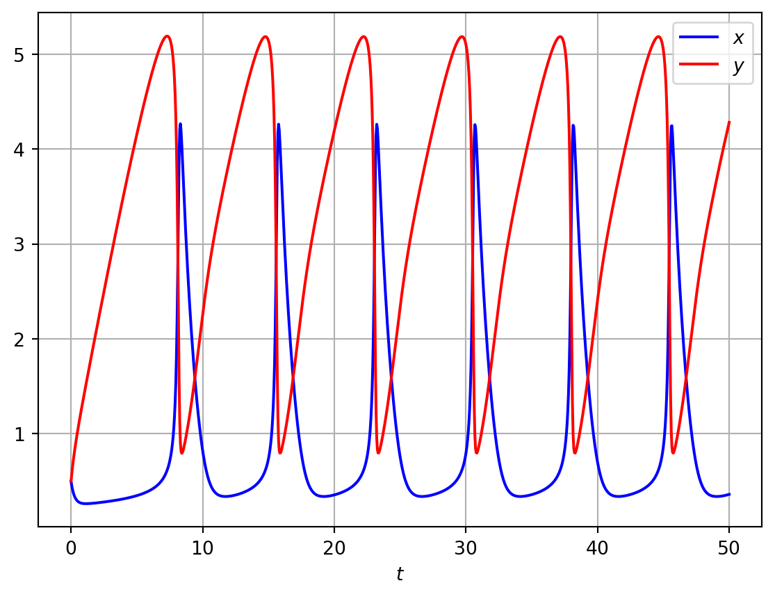
In Figure 5.2 we numerically solve Equation 5.4 in the case of oscillatory solutions. Note that when the steady state is unstable, the numerical solution indicates that the system has limit cycle solutions. A valid question to ask is whether one can prove that this is the case.

import numpy as np
import matplotlib.pyplot as plt
import scipy
from scipy.integrate import odeint

# Define model parameters
a=1.0
b=3.2

# Compute RHS of the brusselator model
def rhs_bruss_model(z,t):
  rhs=np.zeros_like(z)
  x=z[0]
  y=z[1]
  dx_dt=a-b*x+x**2*y-x
  dy_dt=b*x-x**2*y
  rhs[0]=dx_dt
  rhs[1]=dy_dt
  return rhs

# Define time domain and discretise
t = np.linspace(0, 50, 1000)

# Define ICs
init_cond=[0.5,0.5]

# Integrate ODEs
sol1 = odeint(rhs_bruss_model, init_cond,t)

# Plotmresults
x=sol1[:,0]
y=sol1[:,1]

fig, ax= plt.subplots()
ax.plot(t, x, 'b',t,y,'r')
ax.legend(['$x$','$y$'],loc='best')
ax.set_xlabel('$t$')
plt.grid()
plt.show()

Figure 5.2: Numerical solutions of the Brusselator model

5.3.5 Applying the Poincaire-Bendixson theorem

Recall that the Poincaire-Bendixson theorem can be used to prove the existence of limit cycle solutions in a case where a bounding set encloses a single unstable steady state. Hence given the case of the Brusselator with \(b>a^2+1\), the identification of a bounding set will allow application of the Poincaire-Bendixson theorem and hence prove the existence of limit cycle solutions.

We begin by defining the nullclines of the system. The \(x\) nullcline is given by

\[ y=\frac{1+b}{x}-\frac{a}{x^2}. \]

The \(y\) nullclines are given by

\[ y=\frac{b}{x} \ \ \ \textrm{and} \ \ \ x=0. \]

In the positive quadrant, this nullcline has a single root at \(a/(1+b)\), tends to 0 as \(x\rightarrow \infty\) and has a maximum at \(x=2a/(1+b)\).

import numpy as np
import matplotlib.pyplot as plt
import scipy
from scipy.integrate import odeint


# Discretise x for plotting nullclines
x_vec=np.linspace(0.01,6,100)

# COmpute quantities needed for pahse plane
def ComputeBrusselatorSol(a,b,x_vec):
    t = np.linspace(0, 10, 1000)

    # Define different ICs
    init_cond1=[0.75,0.75]
    init_cond2=[4.55,4.15]
    init_cond3=[2.5,0.5]
    # steady state
    ss=[a,b/a]

    # Integrate ODEs
    alpha=2.0
    sol1 = odeint(rhs_bruss_model, init_cond1,t)
    sol2 = odeint(rhs_bruss_model, init_cond2,t)
    sol3 = odeint(rhs_bruss_model, init_cond3,t)



    # Compute nullclines
    x_ncline=(1+b)/x_vec-a/x_vec**2
    y_ncline_1_a=[0,0]    
    y_ncline_1_b=[0,5]   
    y_ncline_2_x=b/x_vec

    return sol1,sol2,sol3,ss,x_ncline,y_ncline_1_a,y_ncline_1_b,y_ncline_2_x


# Compute quantitied
a=1.0
b=3.2
sol1,sol2,sol3,ss,x_ncline,y_ncline_1_a,y_ncline_1_b,y_ncline_2_x=ComputeBrusselatorSol(a,b,x_vec)


# PLot results
fig, ax = plt.subplots(1,2)
ax[0].plot(x_vec,x_ncline,'k--')
ax[0].plot(y_ncline_1_a,y_ncline_1_b,'k--')
ax[0].plot(x_vec,y_ncline_2_x,'r--')

ax[0].plot(sol1[:,0],sol1[:,1],sol2[:,0],sol2[:,1],sol3[:,0],sol3[:,1])
ax[0].plot(ss[0],ss[1],'k*')
ax[0].set_xlabel('$x$')
ax[0].set_ylabel('$y$')

ax[0].set_xlim([-0.05,6])
ax[0].set_ylim([-0.005,6])

# Try different parameters
a=4.0
b=3.2

# Recompute quantities
sol1,sol2,sol3,ss,x_ncline,y_ncline_1_a,y_ncline_1_b,y_ncline_2_x=ComputeBrusselatorSol(a,b,x_vec)

# PLot results
ax[1].plot(x_vec,x_ncline,'k--')
ax[1].plot(y_ncline_1_a,y_ncline_1_b,'k--')
ax[1].plot(x_vec,y_ncline_2_x,'r--')

ax[1].plot(sol1[:,0],sol1[:,1],sol2[:,0],sol2[:,1],sol3[:,0],sol3[:,1])
ax[1].plot(ss[0],ss[1],'k*')
ax[1].set_xlabel('$x$')
ax[1].set_ylabel('$y$')

ax[1].set_xlim([-0.05,6])
ax[1].set_ylim([-0.005,6])

plt.tight_layout()
plt.grid()
plt.show()

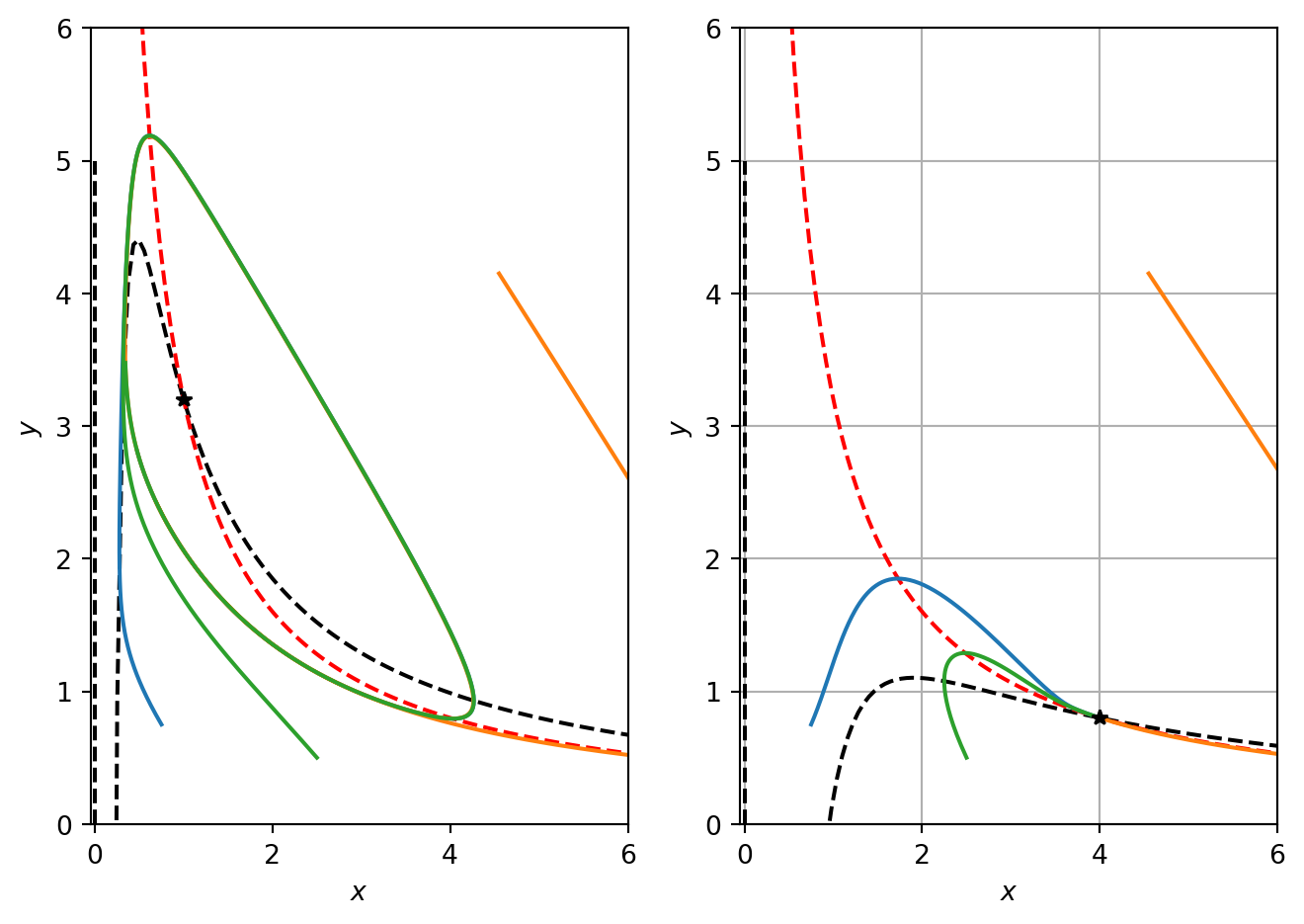
Figure 5.3: Numerical solution of the Brusselator.

In Figure 5.3 we plot the the oscillatory solution together with the nullclines. Note that the nullclines separate the phase plane into regions of constant sign. Note that the \(x\) nullcline separates the phase plane into regions where \(dx/dt>0\) and \(dx/dt<0\). Similarly, the \(y\) nullcline separates the phase plane into regions where \(dy/dt>0\) and \(dy/dt<0\).

Note that signs for \(dx/dt\) can be determined by considering behaviour of the function \(f\) as one moves away from the nullcline where, by definition, \(f=0\). Consider some point that sits on the x nullcline. While keeping the \(x\) value fixed, increase \(y\) so the point moves vertically in the phase plane. This implies that \(f\) has increased because the only term to change is \(x^2y\). Hence \(f\) increases upon increasing \(y\) and therefore \(dx/dt\) is positive for all points above the \(x\) nullcline. Alternatively, note that in the Jacobian matrix we have calculated that \(\partial f/\partial y\) is positive.

5.3.5.1 A confined set

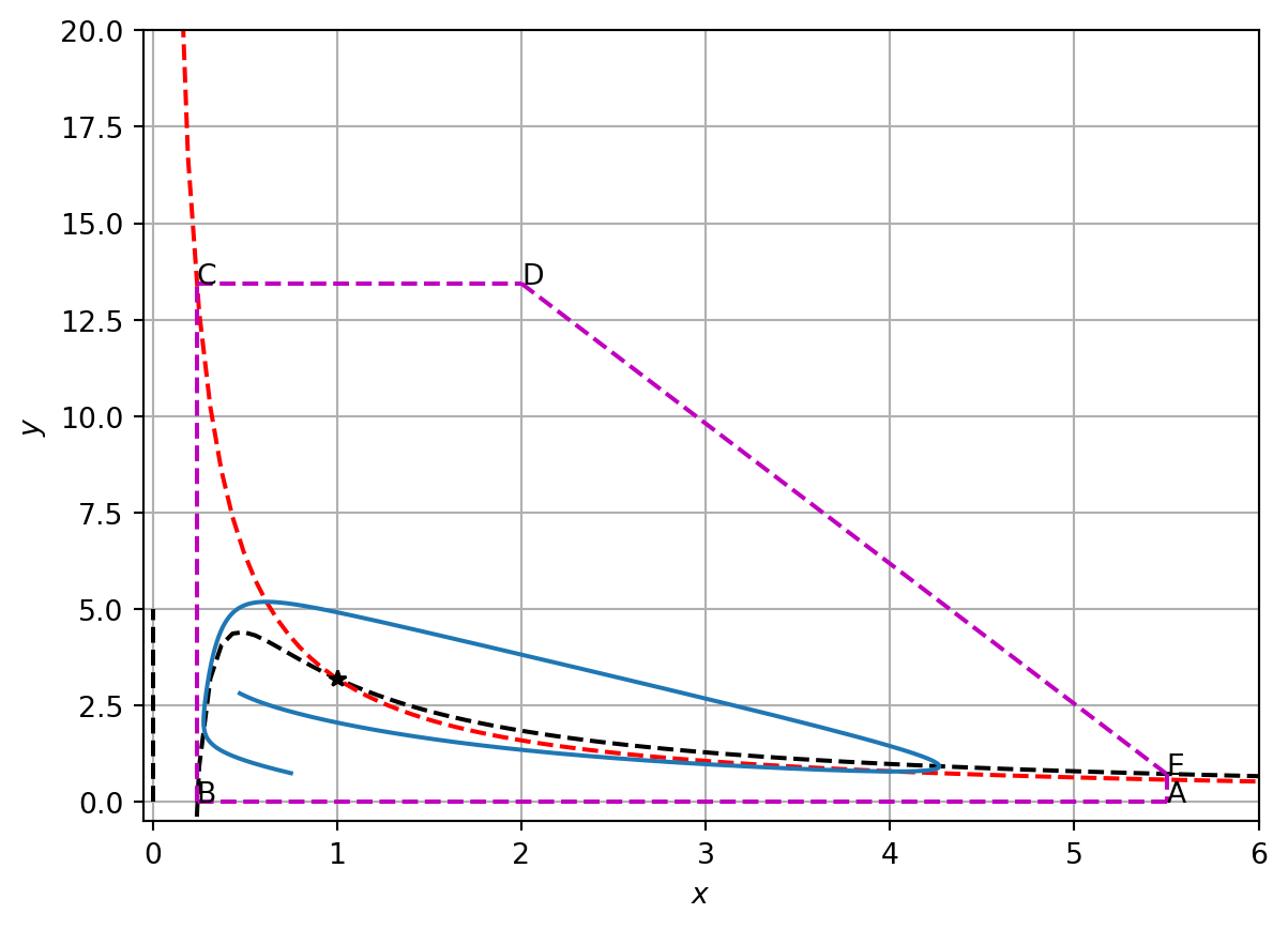
To define a confined set, we construct the closed loop ABCDEA in phase space (see Figure 5.4) where the points A, B, C, D and E are defined as follows. Let the points A and B be two points on the \(x\) axis with coordinates \[ (\delta,0) \] and \[ \left(\frac{a}{1+b},0\right). \] respectively. We choose \(\delta>a\). The outward normal to the line segment AB is \(\mathbf{n}=[0,-1]\). To show that the trajectories point inwards along AB, we compute

\[ \mathbf{n}.\left[\frac{dx}{dt},\frac{dy}{dt}\right] = -\frac{dy}{dt}. \]

As the line segment AB sits below the \(y\) nullcline, \(dy/dt>0\) in this region. Hence

\[ \mathbf{n}.\left[\frac{dx}{dt},\frac{dy}{dt}\right] = -\frac{dy}{dt}<0. \]

Hence trajectories point inwards on the line segment AB.

Let \(C\) represent the point \[ \left(\frac{a}{1+b},b\frac{1+b}{a}\right). \]

The normal vector to the line segment BC is \(\mathbf{n}=[-1,0]\). As BC lies to the left of the \(x\) nullcline, in a region where \(dx/dt>0\), then

\[ \mathbf{n}.\left[\frac{dx}{dt},\frac{dy}{dt}\right] = -\frac{dx}{dt}<0. \]

Hence trajectories point inwards on the line segment BC.

Consider the line segment CD where D has coordinates \[ \left(k,b\frac{1+b}{a}\right), \] with \(k>a\)

The normal to this line segment is [0,1]. As CD lies in a region of the phase plane where \(dy/dt<0\),

\[ \mathbf{n}.\left[\frac{dx}{dt},\frac{dy}{dt}\right] = \frac{dy}{dt}<0. \] Hence trajectories point inwards on the line segment CD.

Let E be a point that sits on the \(x\) nullcline at some position \[ \left(\delta,\frac{\delta(1+b)-a}{\delta^2}\right), \] such that DE is a straight line with outwardly pointing normal vector \([1,1]\). Along DE

\[ \mathbf{n}.\left[\frac{dx}{dt},\frac{dy}{dt}\right] = a-bx+x^2y-x + bx-x^2y = a-x<0 \]

for \(x>a\). As \(k>a\), \(x>a\) for all points on DE, hence trajectories point inwards on DE.

Finally, consider the line segment EA which has normal vector \(\mathbf{n}=[1,0]\). As \(dx/dt<0\) along EA

\[ \mathbf{n}.\left[\frac{dx}{dt},\frac{dy}{dt}\right] = \frac{dx}{dt} <0. \]

import numpy as np
import matplotlib.pyplot as plt
import scipy
from scipy.integrate import odeint



x_vec=np.linspace(0.01,6,100)

def ComputeCompetitionSol(a,b,x_vec):
    t = np.linspace(0, 10, 1000)

    init_cond1=[0.75,0.75]
    init_cond2=[4.55,4.15]
    init_cond3=[2.5,0.5]

    ss=[a,b/a]

    alpha=2.0
    sol1 = odeint(rhs_bruss_model, init_cond1,t)
    


  
    x_ncline=(1+b)/x_vec-a/x_vec**2
    y_ncline_1_a=[0,0]    
    y_ncline_1_b=[0,5]   
    y_ncline_2_x=b/x_vec

    return sol1,ss,x_ncline,y_ncline_1_a,y_ncline_1_b,y_ncline_2_x

a=1.0
b=3.2
sol1,ss,x_ncline,y_ncline_1_a,y_ncline_1_b,y_ncline_2_x=ComputeCompetitionSol(a,b,x_vec)


k=2*a
delta=5.5

A=[delta,0]
B=[1/(1+b),0]
C=[a/(1+b),b*(1+b)/a]
D=[k,b*(1+b)/a]
E=[delta,(delta*(1+b)-a)/delta**2]


fig, ax = plt.subplots()
ax.plot(x_vec,x_ncline,'k--')
ax.plot(y_ncline_1_a,y_ncline_1_b,'k--')
ax.plot(x_vec,y_ncline_2_x,'r--')

ax.plot(sol1[:,0],sol1[:,1])
ax.plot(ss[0],ss[1],'k*')
ax.plot([A[0], B[0]],[A[1], B[1]],'m--')
ax.plot([B[0], C[0]],[B[1], C[1]],'m--')
ax.plot([C[0], D[0]],[C[1], D[1]],'m--')
ax.plot([D[0], E[0]],[D[1], E[1]],'m--')
ax.plot([E[0], A[0]],[E[1], A[1]],'m--')

ax.annotate('A', A)
ax.annotate('B', B)
ax.annotate('C', C)
ax.annotate('D', D)
ax.annotate('E', E)


plt.xlabel('$x$')
plt.ylabel('$y$')

ax.set_xlim([-0.05,6])
ax.set_ylim([-0.5,20])


plt.grid()
plt.show()

Figure 5.4: Numerical solution of the Brusselator.

Hence at all points on the closed loop ABCDEA trajectories point inwards (see Figure 5.4). Hence ABDCEA is a confined set and the Poincaire-Bendixson theorem states that the system exhibits limit cycle solutions when the steady state is unstable. This is precisely the behaviour that we see numerically in Figure Figure 5.3.