Week 1: Displacement Vectors

The word “vector” can be used to mean slightly different but closely related concepts. Here we use a definition based on physics, and later we will see how this relates to the more general and precise mathematical definition, and also the concept of vectors in computer science.

Scalars are mathematical objects that can be described by a single number. Common examples from physics include temperature, pressure and density. Vectors are defined by two things: a direction and a magnitude. Common examples are displacement, force, acceleration and velocity ¹.

A vector space is associated with a dimension. They can have any integer number of dimensions or even be infinite-dimensional, but in this module we will consider only two- and three-dimensional vectors, which are the ones that we can easily imagine and draw.

In this section of the course we will examine the mathematics of vectors.

Displacements

We proceed initially by considering the particular case of displacement vectors.

We begin by using notation for “directed line segments”: if we start at \(A\) and displace to \(B\), we denote this displacement vector by \({\overrightarrow{AB}}\). The arrow shows the direction and the length is denoted by \(|{\overrightarrow{AB}}|\).

Note that though these are vectors, there are no numbers in this section. Later we will see how this is linked to vector notation, and column vectors, that you may hae seen before.2

An example of a displacement vector is a distance 10 miles in a North-Westerly direction. Note that the displacement vector is not located at a position in space (or on the map) but precisely defines a displacement from any point.

We can define what operations we want our displacements to have, like addition and multiplication. How can we do this in a consistent and intuitive way?

Equality

Two displacements are equal if their lengths and directions are equal.

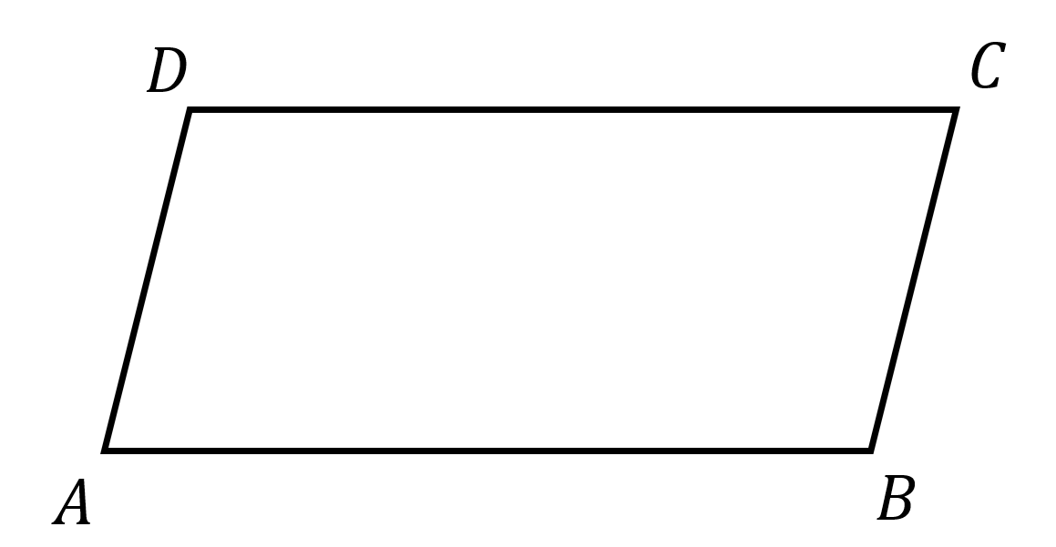
In the diagram Figure 1 below, \({\overrightarrow{AD}} = {\overrightarrow{BC}}\) because the directions and lengths are the same, even though the endpoints are different. On the other hand, \({\overrightarrow{AD}} \ne {\overrightarrow{DA}}\) because even though the lengths are the same, \(|{\overrightarrow{AD}}| = |{\overrightarrow{DA}}|\), the directions are not.

Think: is \({\overrightarrow{AB}}\) equal to \({\overrightarrow{CD}}\) or \({\overrightarrow{DC}}\)?

Solution

\({\overrightarrow{CD}}\) has the opposite direction. \({\overrightarrow{AB}} = {\overrightarrow{DC}}\).

Figure 1: A parallelogram \(ABCD\)

Adding displacements

Adding displacements is easy when the endpoint of the first displacement is the startpoint of the second. Consider this diagram:

Figure 2: A triangle \(ADF\)

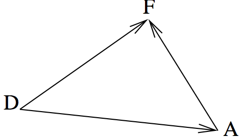
Here we see that going from \(D\) to \(A\) and then from \(A\) to \(F\) is the same as going directly from \(D\) to \(F\). So we write \({\overrightarrow{DA}} + {\overrightarrow{AF}} = {\overrightarrow{DF}}\).

Without knowing anything about the points \(X\), \(Y\) and \(Z\), we can say that \({\overrightarrow{XY}}+{\overrightarrow{YZ}}={\overrightarrow{XZ}}\). We just “cancel” the middle letter.

Note

To add two displacements with a common letter in the midddle, just cancel out that letter.

If there is no common middle letter, then we just need to remember that the displacements do not have a fixed position – we can “move” them. Sometimes it helps if we know other equivalent displacements. For example, in Figure 1, \({\overrightarrow{AD}} + {\overrightarrow{AB}} = {\overrightarrow{AD}} + {\overrightarrow{DC}} = {\overrightarrow{AC}}\).

Think: In Figure 1, what one displacement is equal to \({\overrightarrow{BC}} + {\overrightarrow{DB}}\)?

Solution

\({\overrightarrow{BC}} = {\overrightarrow{AD}}\) so \({\overrightarrow{BC}} +{\overrightarrow{DB}}= {\overrightarrow{AD}} + {\overrightarrow{DB}} = {\overrightarrow{AB}}\)

Triangle inequality

When we add displacements, the length of the result is NOT the two lengths added together, in general. It is not true that \(|{\overrightarrow{DA}}|+|{\overrightarrow{AF}}|=|{\overrightarrow{DF}}|\). In fact, thinking about Figure 2 we can see that \(|{\overrightarrow{DA}}|+|{\overrightarrow{AF}}|\geq|{\overrightarrow{DF}}|\). This is called the triangle inequality.

Addition is commutative

In mathematics we use special words to describe different operations. An operation is commutative if we can swap around the sides and get the same answer. For example, \(2+5 = 5+2\), so normal addition of scalars is commutative. That’s true of vector addition too!

Think: of the other basic operations of scalars, \(-\), \(\times\) and \(\div\), which is commutative and which are not?

Solution

Multiplication is commutative, but subtraction and division are not: \(3-2=1\) but \(2-3=-1\) and \(10\div2 = 5\) but \(2\div10 = 0.2\).

In Figure 1, \({\overrightarrow{AD}} + {\overrightarrow{DC}} = {\overrightarrow{AC}}\), and using the fact that \({\overrightarrow{DC}} = {\overrightarrow{AB}}\) and \({\overrightarrow{AD}} = {\overrightarrow{BC}}\), we see that \({\overrightarrow{DC}} + {\overrightarrow{AD}} = {\overrightarrow{AB}} + {\overrightarrow{BC}} = {\overrightarrow{AC}}\), so we have proven that \({\overrightarrow{AD}} + {\overrightarrow{DC}} = {\overrightarrow{DC}} + {\overrightarrow{AD}}\).

Addition is associative

An operation is associative if it doesn’t matter where we write brackets. For example, \((3+2) + 5 = 3 + (2+5)\). For associative operations, we don’t need to write the brackets at all, and it’s unambiguous to say “three plus five plus two”. (This isn’t true of subtraction. If someone said “ten minus two minus one” would the answer be 7 or 9? \((10-2)-1\) is not the same as \(10-(2-1)\).)

Looking at Figure 1, we see that \(({\overrightarrow{AB}} + {\overrightarrow{BC}}) + {\overrightarrow{CD}} = {\overrightarrow{AC}} + {\overrightarrow{CD}} = {\overrightarrow{AD}}\), and \({\overrightarrow{AB}} + ({\overrightarrow{BC}} + {\overrightarrow{CD}}) = {\overrightarrow{AB}} + {\overrightarrow{BD}} = {\overrightarrow{AD}}\). Therefore, we have proven that \(({\overrightarrow{AB}} + {\overrightarrow{BC}}) + {\overrightarrow{CD}} = {\overrightarrow{AB}} + ({\overrightarrow{BC}} + {\overrightarrow{CD}})\). Addition of displacements is associative.

The zero displacement

With normal scalar numbers, we have the special number \(0\) which we can add to anything and not change the answer. \(3+0=3\), \(0+10=10\), etc.

We define a special displacement, denoted \({\mathbf{0}}\), which we can add to any displacement and not change the answer. \({\overrightarrow{AB}} + {\mathbf{0}} = {\overrightarrow{AB}}\), and also, by commutativity, \({\mathbf{0}} + {\overrightarrow{AB}} = {\overrightarrow{AB}}\). We think of this displacement as starting at any point, and then not moving!

Negative displacements

Every normal positive number has a corresponding negative number, and these have the special property that they add together to give \(0\). That is to say, \(3+(-3) = 0\).

We would like to have the same thing with displacements. What displacement can I add to \({\overrightarrow{AB}}\) to get the zero displacement, i.e. to get back to where I started? Obviously, we should choose \({\overrightarrow{BA}}\). So, \({\overrightarrow{AB}} + {\overrightarrow{BA}} = {\mathbf{0}}\), and we write that \(-{\overrightarrow{BA}} = {\overrightarrow{AB}}\).

Note

To take the negative of a displacement, just swap the letters round.

Subtracting displacements

We define subtraction using the negatives in the obvious way, so \({\overrightarrow{AB}} - {\overrightarrow{CB}} = {\overrightarrow{AB}} + (-{\overrightarrow{CB}}) = {\overrightarrow{AB}} + {\overrightarrow{BC}}\).

Multiplying displacements

For now, let’s ignore the idea of multiplying two displacements together, and instead concentrate on multiplying displacements by scalars.

We can define multiplication by an integer in an obvious way: \[ 3{\overrightarrow{AB}} = {\overrightarrow{AB}} + {\overrightarrow{AB}} + {\overrightarrow{AB}}. \]

Important

For normal numbers \(ab\), \(a\times b\) and \(a\cdot b\) are all the same thing. For vectors, we save the dot and cross for special meanings, and only ever use the first notation for multiplication of a scalar and a vector.

Here the result of \(3{\overrightarrow{AB}}\) is clearly in the same direction as \({\overrightarrow{AB}}\), and it has three times the length. So in general, multiplying by a scalar results in a displacement in the same direction, but with the length changed.

Note

To multiply a displacement by a negative number, first multiply by the positive number and then flip the direction.

Scalar multiplication is distributive over vector addition

Now for some more jargon: an operation are distributive over another operation if we can expand out the brackets. So for normal multiplication and addition, \(3\times(5+2) = 3\times 5+3\times 2\).

What about for displacments? \[ 2{\overrightarrow{AB}} + 2{\overrightarrow{XY}} = {\overrightarrow{AB}} + {\overrightarrow{AB}} + {\overrightarrow{XY}} + {\overrightarrow{XY}} = ({\overrightarrow{AB}} + {\overrightarrow{XY}}) + ({\overrightarrow{AB}} + {\overrightarrow{XY}}) = 2({\overrightarrow{AB}}+{\overrightarrow{XY}}). \]

Think: which of the other rules have we used in this derivation?

Solution

To write \({\overrightarrow{AB}} + {\overrightarrow{AB}} + {\overrightarrow{XY}} + {\overrightarrow{XY}} = {\overrightarrow{AB}} + {\overrightarrow{XY}} + {\overrightarrow{AB}} + {\overrightarrow{XY}}\), we have used commutativity of addition. To add the brackets in, we used associativity.

Figure 3: The vector \({\overrightarrow{AC}}\) is twice the length of \({\overrightarrow{AB}}\) and in the same direction, so \({\overrightarrow{AC}}=2{\overrightarrow{AB}}\).

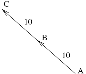
In Figure 3, we see that \({\overrightarrow{BC}}={\overrightarrow{AB}}\), so \({\overrightarrow{AC}}={\overrightarrow{AB}}+{\overrightarrow{BC}}=2{\overrightarrow{AB}}\).

Dividing by a scalar

We’ve defined addition, subtraction and multiplication. What about division? To divide a vector by \(2\), just multiply by \(\frac{1}{2}\).

Colinear points

Three (or more) points are colinear (they lie on the same line) if all the vectors between them are in the same or opposite directions, i.e. they can all be written as scalar multiples of each other.

In Figure 3, points \(A\), \(B\) and \(C\) are colinear because \({\overrightarrow{AC}}=2{\overrightarrow{AB}}\), or alternatively \({\overrightarrow{CA}}=2{\overrightarrow{CB}}\).

Examples for displacements

Example: Colinear points

Let \(A,B,C\) be colinear, and \({\overrightarrow{AB}} = \alpha {\overrightarrow{AC}}\), for \(0 < \alpha < 1\).

Also, let \(|{\overrightarrow{AB}}| = \lambda\) and \(|{\overrightarrow{BC}}| = \mu\).

Find \(\alpha\) in terms of \(\lambda\) and \(\mu\).

Figure 4

Solution

From Figure 4 we see that \(|{\overrightarrow{AC}}| = \lambda+ \mu\). What is \(\alpha\)?

Now \(| {\overrightarrow{AB}} | = \alpha |{\overrightarrow{AC}}|\), so that Thus \({\overrightarrow{AB}}= \left(\frac{\lambda}{\lambda+ \mu}\right) {\overrightarrow{AC}}\). Similary \({\overrightarrow{BC}}= \left(\frac{\mu}{\lambda+ \mu}\right) {\overrightarrow{AC}}\).

Example: Parallelogram

Let \(RSTU\) be a parallelogram (see Figure 5), and extend \(RU\) to \(A\) so that \({\overrightarrow{RU}} = {\overrightarrow{UA}}\). Also let \(C\) be the mid-point of \(UT\). Prove that \(C\) is the midpoint of \(SA\).

Figure 5

Solution

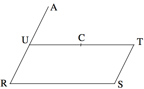
We have \[{\overrightarrow{SA}} = {\overrightarrow{SR}} + {\overrightarrow{RA}} = {\overrightarrow{TU}} + {\overrightarrow{RA}} = 2\,{\overrightarrow{CU}} + 2\, {\overrightarrow{UA}} = 2 ({\overrightarrow{CU}}+{\overrightarrow{UA}})= 2\, {\overrightarrow{CA}}. \] Thus \(S,C,A\) are colinear, and \(C\) is the mid-point of \(SA\).

Footnotes

1. In common language, we use “speed” and “velocity” interchangeably. In physics, velocity is a vector quantity and speed is a scalar, the magnitude of the velocity.