Infectious disease

Infectious diseases can have severe health outcomes for individuals who contract them. They can also place an unmanageably large demand on the health service.

Infectious diseases can be characterised using their basic reproduction number, \(R_0\).

Infectious disease basic reproduction numbers Source.
Disease	\(R_0\)
Measles	12-18
Chickenpox	10-12
Rubella	6-7
Common cold	2-3
Covid 19 (Omicron)	9.5

Mathematical modelling of infectious diseases

We can use mathematics to study the dynamics of an infectious disease within a population. In the SIR model a population is split into three compartments:

\(S(t)\) - size of susceptible population at time \(t\)
\(I(t)\) - size of infected population at time \(t\)
\(R(t)\) - size of recovered/post-infected population at time \(t\)

The SIR model has two parameters:

\(r\) - infection rate
\(a\) - recovery rate

From a public health perspective, one could propose that there is some level of infectiousness, \(I_{max}\), which must be avoided. The challenge is to manage the disease such that \(I(t)<I_{max}\) for all \(t\).

In the app in Figure 1 you can investigate how the values of the parameters \(r\) and \(a\) affect the trajectory of the infectious disease.

Tip

Please note that the app in Figure 1 is approximately 20 MB. If it does not display on your device:

wait a few moments (it is downloading the Python code that will run the app)
refresh your browser.
try running on a faster connection/ more powerful device.

If it still does not load, here is a screenshot.

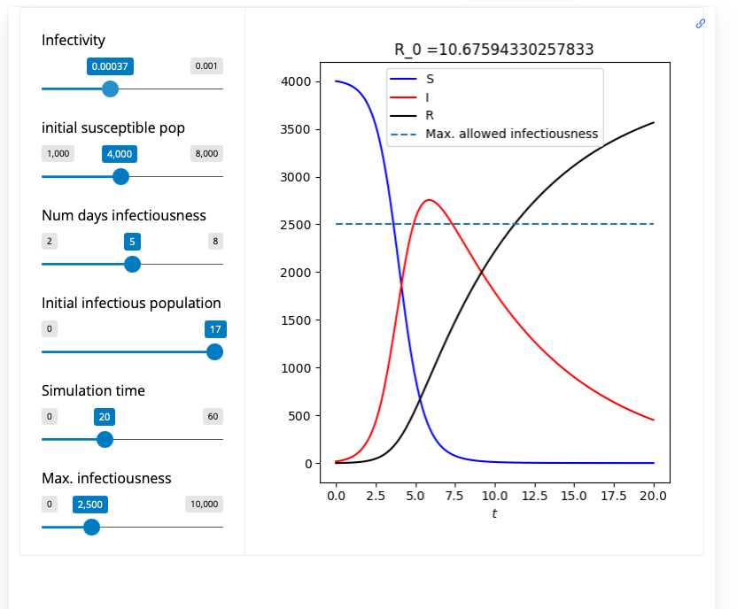
#| standalone: true
#| components: [viewer]
#| viewerHeight: 800

from shiny import App, Inputs, Outputs, Session, render, ui
from shiny import reactive

import numpy as np
from pathlib import Path
import matplotlib.pyplot as plt
from scipy.integrate import odeint

app_ui = ui.page_fluid(
    ui.layout_sidebar(
        ui.panel_sidebar(
    ui.input_slider(id="r",label="r",min=0.00001,max=0.001,value=0.001,step=0.00001),
    ui.input_slider(id="S0",label="Initial susceptible pop. (S(0))",min=1000.0,max=8000.0,value=4000.1,step=5.0),
    ui.input_slider(id="a",label="a",min=0.01,max=0.2,value=0.05,step=0.001),            
    ui.input_slider(id="I0",label="Initial infectious pop. (I(0)) ",min=0.0,max=17.0,value=17.0,step=0.5),  
    ui.input_slider(id="T",label="Simulation time",min=0.0,max=70.0,value=40.0,step=0.5),
    ui.input_slider(id="max_inf",label="Max. infectiousness",min=0.0,max=10000.0,value=2500.0,step=100.5),             
          
            ),

        ui.panel_main(ui.output_plot("plot"),),
    ),
)

def server(input, output, session):
    
    @render.plot
    def plot():
        fig, ax = plt.subplots()
        #ax.set_ylim([-2, 2])
        # Filter fata
        
        
        r=float(input.r())
        S_0=float(input.S0())
        a=float(input.a())
        I_0=float(input.I0())
        T=float(input.T())
        max_inf=float(input.max_inf())

        R_0=r*S_0/a
        
        # Define rhs of LV ODEs
        def rhs_sir_model(x,t,r,a):
          rhs=np.zeros_like(x,dtype=float)
          S=x[0]
          I=x[1]
          R=x[2]

          

          dS_dt=-r*I*S
          dI_dt=r*I*S-a*I
          dR_dt=a*I

          rhs[0]=dS_dt
          rhs[1]=dI_dt
          rhs[2]=dR_dt

          return rhs

        # Define discretised t domain
        t = np.linspace(0, T, 1000)

        # define initial conditions
        init_cond=[S_0,I_0,0.0]
        
        # Compute numerical solution of ODEs
        sol1 = odeint(rhs_sir_model, init_cond,t,args=(r,a))

        # Plot results
        S=sol1[:,0]
        I=sol1[:,1]
        R=sol1[:,2]
        
        ax.plot(t, S, 'b',t,I,'r',t,R,'k')
        ax.plot(t,max_inf*np.ones_like(t),'--')
        ax.legend(['S','I','R','Max. allowed infectiousness'],loc='best')
        ax.set_xlabel('$t$')
        ax.set_title('R_0 =' + str(R_0))

        #plt.grid()
        #plt.show()
    
app = App(app_ui, server)

Figure 1: The sizes of the different populations are plotted against time, \(t\). The model parameters are defined using the sliders on the left-hand side. The differential equations are in Equation 1.

Exercises with the app

can you determine what value the infectivity parameter, \(r\), must go below in order that \(I(t)<I_{max}\)?
suppose that covid omicron in a susceptible population of \(S_0=5000\) has a recovery rate \(a=0.05\). Can you estimate the value of the infectivity parameter, \(r\), such that \(R_0=9.5\)?
which parameters in the app best represent the effect of vaccination of a section of the population?

The SIR model equations

The SIR model is formulated as a system of ordinary differential equations.

On this page we consider a simpler case of a single population.

The governing equations in the SIR model are: \[ \begin{aligned} \frac{dS}{dt}&=-rIS, \\ \frac{dI}{dt}&=rIS-aI, \\ \frac{dR}{dt}&=aI. \end{aligned} \tag{1}\]

The initial conditions are:

\[ \begin{aligned} S(t=0)&=S_0, \\ I(t=0)&=I_0, \\ R(t=0)&=R_0. \end{aligned} \]

In the app in Figure 1 Equation 1 are solved numerically for a given parameter set and the solution is plotted.

Note

At Dundee, the mathematical tools needed are developed in modules:

Maths 1A, 1B, 2A and 2B (Core maths modules)
Computer algebra and dynamical systems
Mathematical Biology I
Mathematical Biology II

At Levels 2, 3 and 4 you will learn how to use computer programming to explore and communicate mathematical concepts.

You can find out more about these modules here.