Roots of quadratic and cubic equations

Consider the cubic equation \[ ax^3+bx^2+cx+d=0, \ \ \quad a,b,c, d \in \Re. \tag{1}\]

A special case you may have seen before occurs when \(a=0\). Hence \[ bx^2+cx+d=0. \]

In this case the roots of the quadratic are \[ x=\frac{-c\pm\sqrt{c^2-4bd}}{2b}. \]

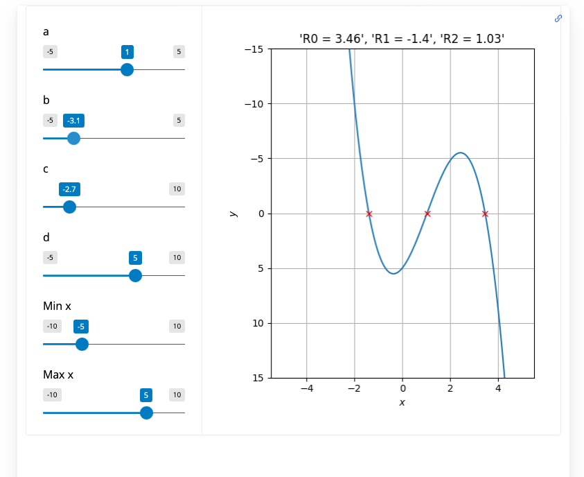
In the app in Figure 1 you can play with the parameter \(a\), \(b\), \(c\) and \(d\) and explore how they affect the form of the cubic equation Equation 1.

Tip

Please note that the app in Figure 1 is approximately 20 MB. If it does not display on your device:

wait a few moments (it is downloading the Python code that will run the app)
refresh your browser.
try running on a faster connection/ more powerful device.

If it still does not load, here is a screenshot.

#| standalone: true
#| components: [viewer]
#| viewerHeight: 800

from shiny import App, Inputs, Outputs, Session, render, ui
from shiny import reactive

import numpy as np
from pathlib import Path
import matplotlib.pyplot as plt

app_ui = ui.page_fluid(
    ui.layout_sidebar(
        ui.panel_sidebar(
    ui.input_slider(id="a",label="a",min=-5,max=5,value=1.0,step=0.1),
    ui.input_slider(id="b",label="b",min=-5.0,max=5.0,value=1.0,step=0.1),
    ui.input_slider(id="c",label="c",min=-5.0,max=10.0,value=5.0,step=0.1),            
    ui.input_slider(id="d",label="d",min=-5.0,max=10.0,value=5.0,step=0.1),            
    ui.input_slider(id="min_x",label="Min x ",min=-10.0,max=10.0,value=-5.0,step=0.1),  
    ui.input_slider(id="max_x",label="Max x",min=-10.0,max=10.0,value=5.0,step=0.1),
        
            ),

        ui.panel_main(ui.output_plot("plot"),),
    ),
)

def server(input, output, session):
    
    @render.plot
    def plot():
        fig, ax = plt.subplots()
        #ax.set_ylim([-2, 2])
        # Filter fata
        
        
        a=float(input.a())
        b=float(input.b())
        c=float((input.c()))
        d=float((input.d()))

        min_x=float(input.min_x())
        max_x=float(input.max_x())

        
        # Define rhs of LV ODEs
        def rhs(x,a,b,c,d):
          rhs=np.zeros_like(x,dtype=float)
          rhs=a*x**3+b*x**2+c*x+d

          return rhs

        # Define discretised t domain
        x = np.linspace(min_x, max_x, 1000)

        # define initial conditions
        
        # Compute numerical solution of ODEs
        y = rhs(x,a,b,c,d)

        coeff=[a,b,c,d]
        roots=np.roots(coeff)

        roots=np.round(roots,2)
        ax.plot(x, y,np.real(roots),np.zeros_like(np.real(roots)),'rx')
        ax.set_xlabel('$x$')
        ax.set_ylabel('$y$')
        y_lim_p=-15.0 #np.min([100,np.max(y)])
        y_lim_m=15.0 #np.max([-100,np.min(y)])

        ax.set_ylim([y_lim_m,y_lim_p])
        ax.invert_yaxis()
        ax.grid()

        text_x=0.25*(min_x+max_x)
        text_y=np.mean(y)
        #title_Str= = ' '.join(map(str, (roots)))
        title_Str=[("R"+ str(j) +" = " + str(roots[j]) ) for j in range(len(roots))]
        title_Str = str(title_Str)[1:-1]

        ax.set_title(title_Str)
        #ax.set_title([("R"+ str(j) +" = " + str(roots[j]) ) for j in range(len(roots))])

        #plt.show()
    
app = App(app_ui, server)

Figure 1: Plot of a cubic function. The roots of the cubic are reported in the figure title. The red crosses depict the real parts of the roots.

Exercises

set \(a=0\).
- how many roots are there?
- how does the local maximum/minimum of the quadratic depend on the sign of the parameter \(b\)?
- why are there complex roots when the condition \(c^2-4bd<0\) is satisfied?
consider the case where \(a>0\).
- how many real roots are there?
- demonstrate that there is always a trivial root (\(x=0\)) in the case \(d=0\).
- demonstrate that in the case \(a=d=1\) with \(b=c=0\) the cubic takes the reduced form \[ x^3=-1. \] Can you show that the roots are \(-1\), \(\frac{1+j\sqrt{3}}{2}\), \(\frac{1-j\sqrt{3}}{2}\) where \(j=\sqrt{-1}\).

Note

At Dundee, you will develop your knowledge in algebra in modules

Maths 1A
Maths 1B
Maths 2A
Maths 2B

At Levels 2, 3 and 4 you will learn how to use computer programming to explore and communicate mathematical concepts.

You can find out more about these modules here.