Intersecting lines in two dimensional space
Consider the equations of two straight lines given by \[ y=m_1x+c_1 \tag{1}\] and \[ y=m_2x+c_2, \tag{2}\] where \(m_1\), \(m_2\), \(c_1\) and \(c_2\) are constants.
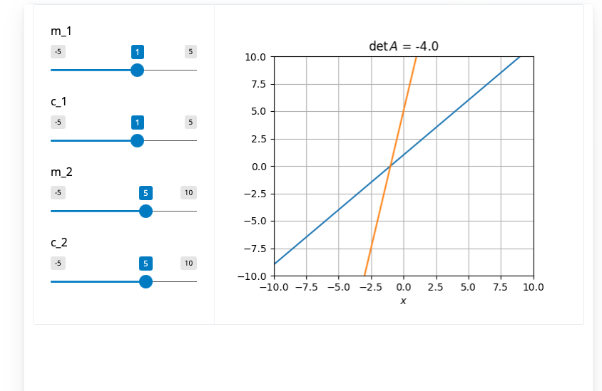
In Figure 1 you can play with the slopes and intercepts of the lines. Can you spot a condition that holds on the slopes such that the straight lines do not intersect?
Problems such as the intersection of straight lines can be formulated using linear algebra. In the title of Figure 1 the determinant of a matrix (defined below) is reported for given values of the slopes and intercept. Can you spot a relationship between the value of the matrix determinant and the geometric properties of the lines?
Please note that the app in Figure 1 is approximately 20 MB. If it does not display on your device:
- wait a moment (it is downloading the Python code that will run the app)
- refresh your browser.
If it still does not load, here is a screenshot.
#| standalone: true
#| components: [viewer]
#| viewerHeight: 500

from shiny import App, Inputs, Outputs, Session, render, ui
from shiny import reactive

import numpy as np
import matplotlib.pyplot as plt

app_ui = ui.page_fluid(
    ui.layout_sidebar(
        ui.panel_sidebar(
    ui.input_slider(id="m_1",label="m_1",min=-5,max=5,value=1.0,step=0.2),
    ui.input_slider(id="c_1",label="c_1",min=-5.0,max=5.0,value=1.0,step=0.2),
    ui.input_slider(id="m_2",label="m_2",min=-5.0,max=10.0,value=5.0,step=0.2),
    ui.input_slider(id="c_2",label="c_2",min=-5.0,max=10.0,value=5.0,step=0.2),
    ),
    ui.panel_main(ui.output_plot("plot"),),
    ),
)

def server(input, output, session):

    @render.plot
    def plot():
        fig, ax = plt.subplots()

        m_1=float(input.m_1())
        c_1=float(input.c_1())
        m_2=float((input.m_2()))
        c_2=float((input.c_2()))

        # Define discretised t domain
        x = np.linspace(-10, 10, 100)
        y_1 = m_1*x+c_1
        y_2 = m_2*x+c_2

        ax.plot(x, y_1, x,y_2)
        matrix=np.zeros((2,2))
        matrix[0,0]=m_1
        matrix[0,1]=1.0
        matrix[1,0]=m_2
        matrix[1,1]=1.0

        matrix=np.matrix(matrix)

        determinant=np.linalg.det(matrix)
        ax.set_title('$\det{A}$ = ' +str(determinant))
        ax.set_ylim([-10,10])
        ax.set_xlim([-10,10])
        ax.grid(True)
        ax.set_xlabel('$x$')
        ax.set_ylabel('$y$')

app = App(app_ui, server)To find the intersection of the lines we can rearrange Equation 1 and Equation 2 to obtain \[ \begin{aligned} m_1x-y&=-c_1, \\ m_2x-y&=-c_2. \end{aligned} \] The equations can be written in matrix-vector form as \[ A \mathbf{x}=\mathbf{b}, \] where \[ A=\begin{pmatrix} m_1 & -1 \\ m_2 & -1\end{pmatrix}, \] and \[ \mathbf{b}=\begin{pmatrix} -c_1 \\ -c_2\end{pmatrix}, \] with \[ \mathbf{x}=\begin{pmatrix} x \\ y\end{pmatrix}. \]
The matrix determinant is defined to be \[ \det{A}=-m_1 +m_2. \]
Hence when the slopes of the lines are equal, the matrix determinant is zero. In this case the lines are parallel and there is either:
- no intersection (the lines have distinct intercepts)
- an infinite family of intersections (the lines also have the same intercept).
Intersecting lines in three dimensional space
We will now explore the intersection of two lines in 3D space.
Consider a line in 3D with direction vector [1,1,1] that passes through the origin. The equation for the line can be written in parametric form as \[ \mathbf{r}_1= \lambda_1 [1,1,1]^T, \quad \lambda_1 \in \Re. \]
Consider a second line defined such that \[ \mathbf{r}_2= \lambda_2 \mathbf{t}+ \mathbf{c}, \quad \lambda_2 \in \Re. \]
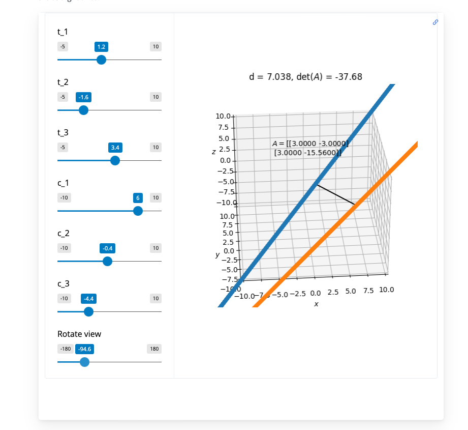
In Figure 2 you can play with the direction vector, \(\mathbf{t}\), and the point \(\mathbf{c}\) of the second line.
In the app set \(c=[c_1,c_2,c_3]^T=[0,0,0]^T\). Can you demonstrate that
- when \(t=[t_1,t_2,t_3]^T=[1,-1,0]^T\) that the lines intersect at the origin?
- when \(t=[t_1,t_2,t_3]^T=[1,1,1]^T\) the minimum distance between the lines is reported as nan (not a number)?
To compute the shortest distance between the two lines we can identify the points on each of the lines (parameters \(\lambda^*\) and \(\mu^*\)) that define closest approach. The equations to define \(\lambda^*\) and \(\mu^*\) can be written in matrix-vector form as \[ A \mathbf{x}=\mathbf{b}, \tag{3}\] where \[ A=\begin{pmatrix} \mathbf{s}\cdot\mathbf{s} & -\mathbf{t}\cdot \mathbf{s} \\ \mathbf{t}\cdot \mathbf{s} & -\mathbf{t}\cdot \mathbf{t}\end{pmatrix}, \] and \[ \mathbf{b}=\begin{pmatrix} \mathbf{c}\cdot \mathbf{s} \\ \mathbf{c}\cdot \mathbf{t}\end{pmatrix}, \] with \[ \mathbf{x}=\begin{pmatrix} \lambda^* \\ \mu^*\end{pmatrix}. \] Here \(\mathbf{s}\) represents the direction vector for the first line.
If a solution to Equation 3 can be found then it is straightforward to calculate the shortest distance, \(d\), between the straight lines.
Please note that the app in Figure 2 is approximately 20 MB. If it does not display on your device:
- wait a moment (it is downloading the Python code that will run the app)
- refresh your browser.
If it still does not work, here is a screenshot.
#| standalone: true
#| components: [viewer]
#| viewerHeight: 800

from shiny import App, Inputs, Outputs, Session, render, ui
from shiny import reactive

import numpy as np
import matplotlib.pyplot as plt

app_ui = ui.page_fluid(
    ui.layout_sidebar(
        ui.sidebar(

    ui.input_slider(id="t_1",label="t_1",min=-5.0,max=10.0,value=5.0,step=0.2),
    ui.input_slider(id="t_2",label="t_2",min=-5.0,max=10.0,value=2.0,step=0.2),
    ui.input_slider(id="t_3",label="t_3",min=-5.0,max=10.0,value=1.0,step=0.2),
    ui.input_slider(id="c_1",label="c_1",min=-10.0,max=10.0,value=-5.0,step=0.2),
    ui.input_slider(id="c_2",label="c_2",min=-10.0,max=10.0,value=5.0,step=0.2),
    ui.input_slider(id="c_3",label="c_3",min=-10.0,max=10.0,value=5.0,step=0.2),
    ui.input_slider(id="azim_ang",label="Rotate view",min=-180.0,max=180.0,value=0.0,step=0.1),
            ),

        ui.output_plot("plot"),
    ),
)


def server(input, output, session):

    @render.plot
    def plot():
        ax = plt.figure().add_subplot(projection='3d')
        #ax.set_ylim([-2, 2])
        # Filter fata

        s_1=1.0
        s_2=1.0
        s_3=1.0

        t_1=float((input.t_1()))
        t_2=float((input.t_2()))
        t_3=float((input.t_3()))
        c_1=float((input.c_1()))
        c_2=float((input.c_2()))
        c_3=float((input.c_3()))
        azim_ang=float((input.azim_ang()))


        # Define discretised t domain

        # L1:r=s*lam+[0,0,0]
        # L2:r=t*lam+[c_1,c_2,c_3]
        #  Define  points on lines (need to used scatter as rendering of plot in 3d using matplotlib id a problem)
        lam=np.linspace(-15.0,15.0,5000)
        L1_x=lam*[s_1]+[0.0]
        L1_y=lam*[s_2]+[0.0]
        L1_z=lam*[s_3]+[0.0]
        L2_x=lam*[t_1]+c_1
        L2_y=lam*[t_2]+c_2
        L2_z=lam*[t_3]+c_3


        # define direction vectors of lines
        c_0_vec=np.array([0,0,0])
        c_2_vec=np.array([c_1,c_2,c_3])
        s_vec=np.array([s_1,s_2,s_3] )
        t_vec=np.array([t_1,t_2,t_3])
        # Find lambdas that define closest point on each lines
        #lam_2=np.dot(c_2_vec-c_0_vec,s_vec-t_vec)/(np.dot(t_vec,t_vec)-np.dot(t_vec,s_vec))

        A=np.array([[np.dot(s_vec,s_vec), -np.dot(t_vec,s_vec)],[np.dot(s_vec,t_vec), -np.dot(t_vec,t_vec)]])
        b=np.array([np.dot(c_2_vec-c_0_vec,s_vec), np.dot(c_2_vec-c_0_vec,t_vec)])

        determinant=np.linalg.det(A)

        #A=np.array([[1,0],[0,1]])
        #b=np.array([1,1])
        x=np.dot(np.linalg.inv(A),b)

        lam_1=x[0]
        lam_2=x[1]

        # Expression for closest points
        cp_1=lam_1*s_vec+c_0_vec
        cp_2=lam_2*t_vec+c_2_vec

        # min distance
        min_dist=np.linalg.norm(cp_2-cp_1)

        #fig = plt.figure()
        ax.scatter(L1_x,L1_y,L1_z)
        ax.scatter(L2_x,L2_y,L2_z,'k*')
        ax.plot([cp_1[0], cp_2[0]],[cp_1[1], cp_2[1]],[cp_1[2], cp_2[2]],'k')
        ax.set_title('d = ' + str(np.round(min_dist,3))+ ', $\det(A)$ = ' + str(np.round(determinant,3)))
        my_matrix=np.array2string(A, suppress_small=True, formatter={'float': '{:0.4f}'.format})

        ax.text(-5,5,5.0, '$A=$'+my_matrix)
        #ax.plot([L2_1[0],L2_2[0]], [L2_1[1],L2_2[1]],[L2_1[2],L2_2[2]],'r',alpha=0.8,linewidth=6)
        ax.set_xlabel('$x$')
        ax.set_ylabel('$y$')
        ax.set_zlabel('$z$')

        ax.set_xlim([-10,10])

        ax.set_ylim([-10,10])
        ax.set_zlim([-10,10])
        #ax.view_init(elev=30, azim=45.0, roll=15)
        ax.view_init(elev=30, azim=azim_ang)

        #determinant=np.linalg.det(matrix)


        #from matplotlib import rc
        #rc('text', usetex=True)
        #my_matrix = "$$A=\\  \\begin{array}{ll} 2 & 3 \\ 4 & 5 \\end{array} \\$$"
        #text(my_matrix, (1,1))

        #ax.text(-10,40, '$A=$'+my_matrix)
        #ax.annotate('$A$ = ' + matrix, xy = (-10, 40), fontsize = 16, xytext = (-10, 40), arrowprops = dict(facecolor = 'red'),color = 'g')


       # ax.annotate(
    #"$\begin{matrix} a & b  \\ d & e  \end{matrix} $",
   # (0.25, 0.25),
   # textcoords='axes fraction', size=20)


        #text_x=0.25*(min_x+max_x)
        #text_y=np.mean(y)
        #title_Str= = ' '.join(map(str, (roots)))
        #title_Str=[("R"+ str(j) +" = " + str(roots[j]) ) for j in range(len(roots))]
        #title_Str = str(title_Str)[1:-1]

        #ax.set_title(title_Str)
        #ax.set_title([("R"+ str(j) +" = " + str(roots[j]) ) for j in range(len(roots))])

        #plt.show()

app = App(app_ui, server)At Dundee, the parametric equations of lines, spheres and planes are studied in the module Maths 1B.
Concepts from geometry and linear algebra are generalised in the modules Maths 2A and Maths 2B.
At Level 3 in the module Differential Geometry geometrical concepts and tools that are essential for understanding classical and modern physics and engineering are further developed.
At Levels 2, 3 and 4 you will learn how to use computer programming to explore and communicate mathematical concepts.
You can find out more about these modules here.