Estimating \(\pi\)
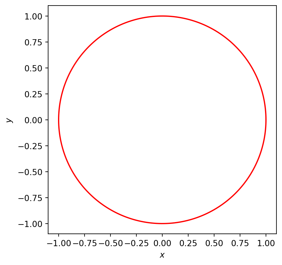
A circle
Consider a circle of radius \(R\) centred at the origin.
The equation of the circle is given by \[ x^2+y^2=R^2. \tag{1}\]
The area of the circle is given by the familiar formula
\[ \pi R^2. \]
The smallest square within which the circle can be inscribed will have side length \(2R\).
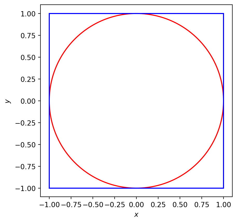
Hence the ratio of the area of the circle to that of the square is
\[ \frac{\pi R^2}{4 R^2}=\frac{\pi}{4}. \]
Estimating \(\pi\)
We can use the above result to estimate \(\pi\) by randomly sampling points that sit inside the square. The probability of a randomly sampled point falling inside the inscribed circle in Figure 2 is equal to the ratio of the areas, i.e. \[ \frac{\pi}{4}. \]
We can use a random number generator to uniformly sample \(N_s\) points within the square, i.e. \[ x_i \in U_{0,2R}, \quad y_i \in U_{0,2R}, \quad i=1,..,N. \] Here \(U\) represents a uniform distribution and \(N\) is the number of sampled points.
We can then count the number of randomly sampled points, \(N_c\), that sit inside the circle, i.e. with coordinates that satisfy the inequality \[ x_i^2+y_i^2< R^2. \]
We can then estimate \(\pi\) using the formula \[ \hat{\pi}\sim 4\frac{N_c}{N_s}. \]
In Figure 3 we use an app to explore the approximation of \(\pi\). Here you can explore how the estimate for \(\pi\) depends on the number of samples and consider circles of different radii.
In the top plot the distribution of sampled points is plotted for a given realisation with the parameter values as you have chosen. In the bottom plot the estimate of \(\pi\) is averaged over different numbers of realisations and plotted against the number of sampled points, \(N\).
#| standalone: true
#| components: [viewer]
#| viewerHeight: 500

from shiny import App, Inputs, Outputs, Session, render, ui
from shiny import reactive

import numpy as np
from pathlib import Path
import matplotlib.pyplot as plt
from scipy.integrate import odeint

app_ui = ui.page_fluid(
    ui.layout_sidebar(
        ui.sidebar(
    ui.input_slider(id="N",label="Num points per experiment (N)",min=10,max=30000,value=10,step=1),
    ui.input_slider(id="R",label="Radius (R)",min=2.0,max=15.0,value=10.0,step=1),
    ui.input_slider(id="L",label="Square side length (L)",min=15.0,max=30.0,value=20.0,step=1),
    ui.input_slider(id="N_Exp",label="Num repeats",min=1,max=300,value=1,step=1),


            ),

        ui.output_plot("plot"),
    ),
)

def server(input, output, session):


    def estimate_pi(N,R,L):
        x = np.random.uniform(0, L, N)
        y = np.random.uniform(0, L, N)

        radius_sq = (x - L/2)**2 + (y - L/2)**2

        num_points_inside_circle = np.sum(radius_sq <= R**2)

        pi_est = (L/R)**2 * (num_points_inside_circle / N)
        return x,y,pi_est

    @render.plot
    def plot():
        fig, ax = plt.subplots(2,1)


        N=int(input.N())
        R=float(input.R())
        L=float(input.L())
        n_samples=int(input.N_Exp())


        x,y,pi_est=estimate_pi(N,R,L)

        radius=((x-L/2)**2+(y-L/2)**2)**(0.5)
        ax[0].plot(x[radius<R],y[radius<R],'b.')
        ax[0].plot(x[radius>R],y[radius>R],'k.')
        ax[0].set_xlabel('$x$')
        ax[0].set_ylabel('$y$')
        ax[0].set_box_aspect(1)
        ax[0].set_xlim([0,L])
        ax[0].set_ylim([0,L])

        theta=np.linspace(0,2*np.pi,1000)
        ax[0].plot(R*np.cos(theta)+L/2.0,R*np.sin(theta)+L/2.0,'r')
        ax[0].set_title('Single realisation, $\hat{\pi}$='+str(round(pi_est,4)))

        N_vec=np.linspace(3,N,30,dtype=int)
        pi_est_vec=np.zeros_like(N_vec,dtype=float)

        # loop over N_vec number of sample points in domain
        for i,N_samp_i in enumerate(N_vec):

            # Try a different sample estimate
            pi_est_i_vec=np.zeros((n_samples,1),dtype=float)
            # Sample pi and store in vector

            for j in range(n_samples):
                x,y,pi_est_ij=estimate_pi(N_samp_i,R,L)
                pi_est_i_vec[j]=(pi_est_ij)
            pi_est_vec[i]=np.mean(pi_est_i_vec)

        ax[1].plot(N_vec,pi_est_vec,'.',N_vec,np.pi*np.ones_like(N_vec))
        ax[1].plot([N,N],[2.5,3.5],'--')
        ax[1].plot(N_vec,np.pi+1/np.sqrt(N_vec),':')
        ax[1].plot(N_vec,np.pi-1/np.sqrt(N_vec),':')

        ax[1].set_xlabel('Num. points per experiment ($N$)')
        ax[1].set_ylabel('$\hat{\pi}$')
        ax[1].set_ylim([2.9,3.3])
        ax[1].set_title('$\hat{\pi}$ average over '+str(n_samples) + ' repeats')
        #plt.Circle([0.0, 0.0 ],R,fill = False,axis=ax)
        #ax.Circle((0.0, 0.0 ),R,fill = False )


        fig.tight_layout()
        plt.grid()
        plt.show()

app = App(app_ui, server)